How the TYPE Function Works
The TYPE function needs to be inputted into a cell in a very specific manner for it to work properly. To manually add this function to a cell needs to be clicked and “=TYPE(” needs to be entered first. After the open parenthesis, a cell reference is used, followed by a closing parenthesis. After the formula is created, the enter button can be pressed to return a number that indicates what type of data is in the cell that was referenced in the function. As stated, there are only six results that the TYPE function can return. Each of these six types of data is defined in detail below: 1 - When the result is a 1 the data referenced is a number. Example: 365 2 - When the result is a 2 the data referenced is text data. Example: Text 4 - When the result is a 4 the data referenced is a logical value. Example: False 16 When the result is a 16 the data referenced is an error value. Example: #DIV/0! 64 When the result is a 64 the data referenced is an array. Example: =TYPE(J5:J9)
Inserting the TYPE Function
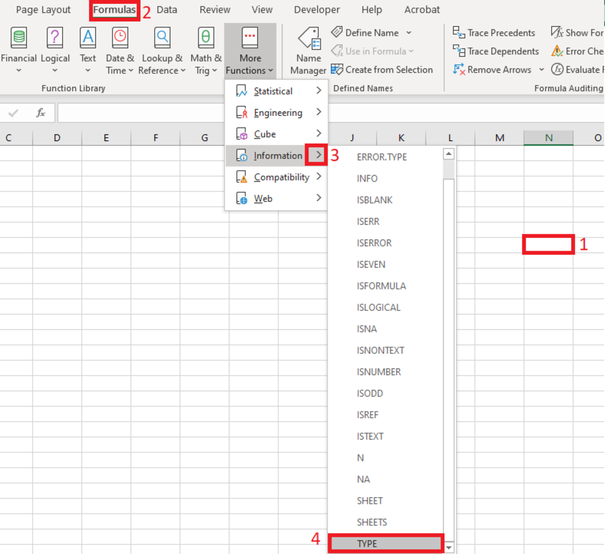
The TYPE function can be inserted into a spreadsheet with the use of an insertion tool. This tool may be preferred by some because of the step-by-step instructions that are given in the process. To insert a function a cell needs to be selected. Next, the formulas tab is selected and the “More Functions” button on the Excel ribbon needs to be selected. The information selection from the list is then chosen, followed by selecting the type option.
Selecting the TYPE Function
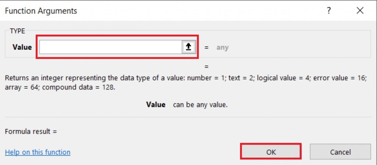
After the function arguments window appears, a cell reference can either be typed or selected from the worksheet by clicking on the up arrow to the right of the value field. Notice the reference under the value field. This reference indicates what value will be returned depending on what type of data is referenced. Once the reference is entered into the value field a preview of the number that will be displayed will appear in the bottom left-hand corner of this window. Additionally, any data can be entered into the values field to see what type of data it is. After the reference is selected, click on the OK button.
The Function Arguments Window For the TYPE Function
TYPE Function Examples
=TYPE(A2) This TYPE formula in the above example will display the type of value in cell A2. If the type of data in cell reference A2 were a name such as Joshua, then the number 1 would appear in the cell where this formula is used. =TYPE(“London”&A3) Returns the type of London, which is text. =TYPE(A4+5) Returns the type of formula in b4 which is 16 the type of error message #VALUE! =TYPE({1,2,3,4}) In this TYPE function, the number 64 is returned since there is an array constant. Any cell that has compound data as such will return this number. =TYPE(10/2) Here a calculation is made where the number 1 is returned since a number would be a result of the calculation. This content is accurate and true to the best of the author’s knowledge and is not meant to substitute for formal and individualized advice from a qualified professional. © 2020 Joshua Crowder